Linear Regression Gradient descent method

Implement multiple linear regression techniques on the Boston house pricing dataset using Scikit-learn.

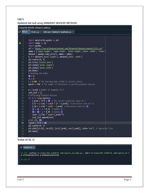
import matplotlib.pyplot as plt
import numpy as np
import pandas
url = “https://raw.githubusercontent.com/jbrownlee/Datasets/master/iris.csv"
names = [‘sepal-length’, ‘sepal-width’, ‘petal-length’,’petal- width’, ‘class’]
dataset = pandas.read_csv(url, names = names)
X, Y = dataset[‘petal-length’], dataset[‘petal- width’]
plt.scatter(X, Y)
plt.title(‘Scatter plot’)
plt.xlabel(‘petal length’)
plt.ylabel(‘petal width’)
plt.show()
# Building the model
t0 = 0
t1 = 0
L = 0.001 # The learning Rate (ALPHA in lecture notes)
epochs = 500 # The number of iterations to perform gradient descent

m = len(X) # Number of examples in X
cost_list = []
# Performing Gradient Descent
for i in range(epochs):
Y_pred = t1*X + t0 # The current predicted value of Y
D_t1 = (-1/m) * sum(X * (Y — Y_pred)) # Derivative term wrt t1
D_t0 = (-1/m) * sum(Y — Y_pred) # Derivative term wrt t0
t1 = t1 — L * D_t1 # Update t1
t0 = t0 — L * D_t0 # Update t0
cost= (1/2*m) * sum(Y-Y_pred)**2
cost_list.append(cost)
print (t1, t0)
Y_pred = t1*X + t0
plt.scatter(X, Y)
plt.plot([min(X), max(X)], [min(Y_pred), max(Y_pred)], color=’red’) #regression line
plt.show()

Output:

plt.plot(list(range(epochs)), cost_list, ‘-r’) #plot the cost function.