linear regression techniques on the Boston house pricing dataset

Implement multiple linear regression techniques on the Boston house pricing dataset using Scikit-learn.

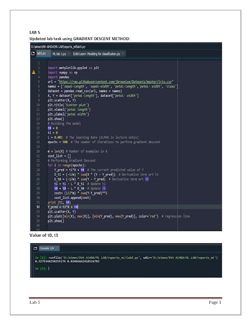
Linear Regression Gradient descent method

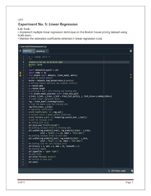
Implement multiple linear regression techniques on the Boston house pricing dataset using Scikit-learn.

import matplotlib.pyplot as plt
import numpy as np
import pandas
url = “https://raw.githubusercontent.com/jbrownlee/Datasets/master/iris.csv"
names = [‘sepal-length’, ‘sepal-width’, ‘petal-length’,’petal- width’, ‘class’]
dataset = pandas.read_csv(url, names = names)
X, Y = dataset[‘petal-length’], dataset[‘petal- width’]
plt.scatter(X, Y)
plt.title(‘Scatter plot’)
plt.xlabel(‘petal length’)
plt.ylabel(‘petal width’)
plt.show()
# Building the model
t0 = 0
t1 = 0
L = 0.001 # The learning Rate (ALPHA in lecture notes)
epochs = 500 # The number of iterations to perform gradient descent

m = len(X) # Number of examples in X
cost_list = []
# Performing Gradient Descent
for i in range(epochs):
Y_pred = t1*X + t0 # The current predicted value of Y
D_t1 = (-1/m) * sum(X * (Y — Y_pred)) # Derivative term wrt t1
D_t0 = (-1/m) * sum(Y — Y_pred) # Derivative term wrt t0
t1 = t1 — L * D_t1 # Update t1
t0 = t0 — L * D_t0 # Update t0
cost= (1/2*m) * sum(Y-Y_pred)**2
cost_list.append(cost)
print (t1, t0)
Y_pred = t1*X + t0
plt.scatter(X, Y)
plt.plot([min(X), max(X)], [min(Y_pred), max(Y_pred)], color=’red’) #regression line
plt.show()

Output:

plt.plot(list(range(epochs)), cost_list, ‘-r’) #plot the cost function.

Logistic Regression

 

Apply the Logistic Regression on ‘weather.csv’ database.

Implement KNN

 

Implement KNN on any data set and choose different values of K to see how it impacts the accuracy of the predictions.

Linear Discriminant Analysis in Python

Linear Discriminant Analysis and comparison with Principle component Analysis in python

Quadratic Discriminant Analysis in PYTHON

Implement QDA on any dataset and explain with comments. Each student should implement on different dataset.

Dataset: Breast cancer

Scikit-Learn | PCA

 

Implementing PCA in Python with Scikit-Learn on Iris dataset.

Step 01: importing required libraries

import numpy as np

import matplotlib.pyplot as plt

import pandas as pd

from sklearn import datasets

Step 02: importing or loading the datasets

dataset = datasets.load_iris()

Step 03: distributing the dataset into two components X and Y

X = dataset.data ; y = dataset.target

Step 04: Splitting the X and Y into the Training set and Testing set

from sklearn.model_selection import train_test_split

X_train, X_test, y_train, y_test = train_test_split(X, y, test_size = 0.25, random_state = 75)

Step 05: performing preprocessing part

from sklearn.preprocessing import StandardScaler

sc = StandardScaler()

X_train = sc.fit_transform(X_train)

X_test = sc.transform(X_test)

Step 06: Applying PCA function on training and testing set of X component

from sklearn.decomposition import PCA

pca = PCA(n_components = 2)

X_train = pca.fit_transform(X_train)

X_test = pca.transform(X_test)

Step 07: Fitting Logistic Regression To the training set

from sklearn.linear_model import LogisticRegression

classifier = LogisticRegression(random_state = 0)

classifier.fit(X_train, y_train)

Step 08: Predicting the test set result using predict function under LogisticRegression

y_pred = classifier.predict(X_test)

Step 09: making confusion matrix between test set of Y and predicted value.

from sklearn.metrics import confusion_matrix

cm = confusion_matrix(y_test, y_pred)

Step 10: Predicting the training set result through scatter plot

from matplotlib.colors import ListedColormap

X_set, y_set = X_train, y_train

X1, X2 = np.meshgrid(np.arange(start = X_set[:, 0].min() — 1,

stop = X_set[:, 0].max() + 1, step = 0.01),

np.arange(start = X_set[:, 1].min() — 1,

stop = X_set[:, 1].max() + 1, step = 0.01))

plt.contourf(X1, X2, classifier.predict(np.array([X1.ravel(),

X2.ravel()]).T).reshape(X1.shape), alpha = 0.75,

cmap = ListedColormap((‘yellow’, ‘white’, ‘aquamarine’)))

plt.xlim(X1.min(), X1.max())

plt.ylim(X2.min(), X2.max())

for i, j in enumerate(np.unique(y_set)):

plt.scatter(X_set[y_set == j, 0], X_set[y_set == j, 1],

c = ListedColormap((‘red’, ‘green’, ‘blue’))(i), label = j)

plt.title(‘Logistic Regression (Training set)’)

plt.xlabel(‘PC1’) # for Xlabel

plt.ylabel(‘PC2’) # for Ylabel

plt.legend() # to show legend

Step 11: show scatter plot

plt.show()

Step 12: Visualising the Test set results through scatter plot

from matplotlib.colors import ListedColormap

X_set, y_set = X_test, y_test

X1, X2 = np.meshgrid(np.arange(start = X_set[:, 0].min() — 1,

stop = X_set[:, 0].max() + 1, step = 0.01),

np.arange(start = X_set[:, 1].min() — 1,

stop = X_set[:, 1].max() + 1, step = 0.01))

plt.contourf(X1, X2, classifier.predict(np.array([X1.ravel(),

X2.ravel()]).T).reshape(X1.shape), alpha = 0.75,

cmap = ListedColormap((‘yellow’, ‘white’, ‘aquamarine’)))

plt.xlim(X1.min(), X1.max())

plt.ylim(X2.min(), X2.max())

for i, j in enumerate(np.unique(y_set)):

plt.scatter(X_set[y_set == j, 0], X_set[y_set == j, 1],

c = ListedColormap((‘red’, ‘green’, ‘blue’))(i), label = j)

Step 13: title for scatter plot

plt.title(‘Logistic Regression (Test set)’)

plt.xlabel(‘PC1’) # for Xlabel

plt.ylabel(‘PC2’) # for Ylabel

plt.legend()

Step 14: show scatter plot

plt.show()

Neural Network

 

Simple Neural Network in Python

Step 01:

import numpy as np

import matplotlib.pyplot as plt # to plot error during training

Step 02: input

inputs=np.array([[0,1,0],

[0,1,1], [1,1,0],[1,0,1]])

Step 03: output

outputs=np.array([[0],[0],[1],[1]])

Step 04: create NeuralNetwork class

class NeuralNetwork:

Step 05: intialize variables in class

def __init__(self, inputs, outputs):

self.inputs = inputs

self.outputs = outputs

Step 06: initialize weights as .50 for simplicity

self.weights = np.array([[.50], [.50], [.50]])

self.error_history = []

self.epoch_list = []

Step 07: activation function ==> S(x) = 1/1+e^(-x)

def sigmoid(self, x, deriv=False):

if deriv == True:

return x * (1 — x)

return 1 / (1 + np.exp(-x))

Step 08: data will flow through the neural network.

def feed_forward(self):

self.hidden = self.sigmoid(np.dot(self.inputs, self.weights))

Step 09: going backwards through the network to update weights

def backpropagation(self):

self.error = self.outputs — self.hidden

delta = self.error * self.sigmoid(self.hidden, deriv=True)

self.weights += np.dot(self.inputs.T, delta)

Step 10: train the neural net for 25,000 iterations

def train(self, epochs=25000):

for epoch in range(epochs):

Step 11: flow forward and produce an output

self.feed_forward()

Step 12: go back though the network to make corrections based on the output

self.backpropagation()

Step 13: keep track of the error history over each epoch

self.error_history.append(np.average(np.abs(self.error)))

self.epoch_list.append(epoch)

Step 14: function to predict output on new and unseen input data

def predict(self, new_input):

prediction = self.sigmoid(np.dot(new_input, self.weights))

return prediction

Step 15: create neural network

NN = NeuralNetwork(inputs, outputs)

Step 16: train neural network

NN.train()

Step 17: create two new examples to predict

example = np.array([[1, 1, 0]])

example_2 = np.array([[0, 1, 1]])

Step 18: print the predictions for both examples

print(NN.predict(example), ‘ — Correct: ‘, example[0][0])

print(NN.predict(example_2), ‘ — Correct: ‘, example_2[0][0])

Step 19: plot the error over the entire training duration

plt.figure(figsize=(15,5))

plt.plot(NN.epoch_list, NN.error_history)

plt.xlabel(‘Epoch’)

plt.ylabel(‘Error’)

plt.show()

 

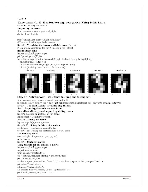
Handwritten digit recognition (Using Scikit-Learn)

Step 001: Loading the Dataset

importing the dataset

from sklearn.datasets import load_digits

digits = load_digits() following command to know the shape of the Dataset:

print(“Image Data Shape” , digits.data.shape)

There are 1797 images in the dataset

Step 002: Visualizing the images and labels in our Dataset

Here we are visualizing the first 5 images in the Dataset

import numpy as np

import matplotlib.pyplot as plt

plt.figure(figsize=(20,4))

for index, (image, label) in enumerate(zip(digits.data[0:5], digits.target[0:5])):

plt.subplot(1, 5, index + 1)

plt.imshow(np.reshape(image, (8,8)), cmap=plt.cm.gray)

plt.title(‘Training: %i\n’ % label, fontsize = 20)

Step 003: Splitting our Dataset into training and testing sets

from sklearn.model_selection import train_test_split

x_train, x_test, y_train, y_test = train_test_split(digits.data, digits.target, test_size=0.05, random_state=95)

Step 004: The Scikit-Learn 4-Step Modeling Pattern

Step 01. Importing the model we want to use.

from sklearn.linear_model import LogisticRegression

Step 02: Making an instance of the Model

logisticRegr = LogisticRegression()

Step 03: Training the Model

logisticRegr.fit(x_train, y_train)

Step 04. Predicting the labels of new data

predictions = logisticRegr.predict(x_test)

Step 05: Measuring the performance of our Model

Use accuracy_score

score = logisticRegr.score(x_test, y_test)

print(score)

Step 06: Confusion matrix

Using Seaborn for our confusion matrix.

import matplotlib.pyplot as plt

import seaborn as sns

from sklearn import metrics

cm = metrics.confusion_matrix(y_test, predictions)

plt.figure(figsize=(9,9))

sns.heatmap(cm, annot=True, fmt=”.3f”, linewidths=.5, square = True, cmap = ‘Pastel1’);

plt.ylabel(‘Actual label’);

plt.xlabel(‘Predicted label’);

all_sample_title = ‘Accuracy Score: {0}’.format(score)

plt.title(all_sample_title, size = 15);